Random effects strategies in `mice.impute.2l.bin`

Stef van Buuren

2026-05-29

Background

mice.impute.2l.bin() imputes a binary outcome in a two-level (clustered) data structure using a logistic mixed model fitted by lme4::glmer(). A key modelling choice is how the cluster-specific random effect $b_i^*$ is drawn for clusters that contain missing values.

Audigier et al. (2018, p. 163) describe two situations for the FCS-GLM imputer:

• Systematic missingness: cluster $i$ has no observed values of $y$. Nothing is known about $b_i$ from the data, so the only coherent draw is from the marginal prior $b_i^* \sim N(0, \psi^*)$.

• Sporadic missingness: cluster $i$ has some observed values of $y$. These observations are informative about $b_i$, so the draw should come from the posterior $p(b_i \mid y_{\text{obs},i}, X_i, \beta^*, \psi^*)$.

mice.impute.2l.bin() exposes three strategies via the random.effects argument.

The three strategies

"marginal" — original behaviour

$$b_i^* \sim N(0, \psi^*)$$

All missing clusters, sporadic or systematic, draw from the marginal prior. This ignores the observed responses within a partially observed cluster.

Pro: Simple; correct for systematic missingness. Con: For sporadic clusters, ignores information in $y_{\text{obs},i}$, leading to overdispersed imputations.

"eb" — Empirical Bayes

$$b_i^* \sim N(\hat{b}_i, \psi^*)$$

The draw is centred on the BLUP $\hat{b}_i$ from lme4::ranef(), but still spread with the full marginal variance $\psi^*$.

Pro: Uses the observed data to locate $b_i^*$; easy to implement. Con: Does not account for the uncertainty in $\hat{b}_i$. Clusters with few observations get the same spread as clusters with many observations, underestimating uncertainty for small clusters and overestimating it for large ones.

"laplace" — Laplace approximation (default)

$$b_i^* \sim N(m_i, V_i)$$

where $m_i$ is the BLUP and $V_i$ is the Laplace-approximated posterior variance returned by lme4::ranef(fit, condVar = TRUE).

As $n_i \to 0$, $V_i \to \psi^*$ and $m_i \to 0$, recovering the marginal draw. As $n_i \to \infty$, $V_i \to 0$ and $m_i \to \hat{b}_i$, concentrating the draw around the BLUP.

Pro: Posterior uncertainty in $b_i$ is correctly reflected; bridges sporadic and systematic cases continuously; consistent with the recommendation of Audigier et al. (2018). Con: Relies on the Laplace approximation, which can be inaccurate for very sparse binary data (few events per cluster).

Simulation

We simulate a two-level dataset with known parameters to make the differences between strategies visible. Strong random effects ($\sigma_b = 3$) and a mix of sporadic and systematic missingness create conditions where the three methods behave differently.

library(mice)
library(ggplot2)

set.seed(42)

# simulate data
n_clusters    <- 60
n_per_cluster <- 8
sigma_b       <- 3
beta0         <- -0.5
beta1         <-  1.0

cluster <- rep(seq_len(n_clusters), each = n_per_cluster)
x1      <- rnorm(n_clusters * n_per_cluster)
b_true  <- rnorm(n_clusters, 0, sigma_b)
logit   <- beta0 + beta1 * x1 + b_true[cluster]
y       <- rbinom(length(logit), 1, plogis(logit))
dat     <- data.frame(cluster = cluster, x1 = x1, y = y)

# systematic missingness: 30% of clusters have all y missing
sys_cl     <- sample(seq_len(n_clusters), 18)
dat$y_miss <- dat$y
dat$y_miss[dat$cluster %in% sys_cl] <- NA

# sporadic missingness: 60% of remaining observations missing
spor_idx <- which(!is.na(dat$y_miss))
dat$y_miss[sample(spor_idx, round(0.6 * length(spor_idx)))] <- NA

n_obs_per_cluster <- tapply(!is.na(dat$y_miss), dat$cluster, sum)
cat(sprintf(
  "Clusters: %d total, %d systematic (all missing), %d sporadic\n",
  n_clusters, length(sys_cl), n_clusters - length(sys_cl)
))
#> Clusters: 60 total, 18 systematic (all missing), 42 sporadic
cat(sprintf(
  "Observed y per sporadic cluster: median %g, range %g-%g\n",
  median(n_obs_per_cluster[n_obs_per_cluster > 0]),
  min(n_obs_per_cluster[n_obs_per_cluster > 0]),
  max(n_obs_per_cluster[n_obs_per_cluster > 0])
))
#> Observed y per sporadic cluster: median 3, range 1-6
cat("True proportion:", round(mean(y), 3), "\n")
#> True proportion: 0.404

pred <- make.predictorMatrix(dat[, c("cluster", "x1", "y_miss")])
pred["y_miss", "cluster"] <- -2
pred["y_miss", "x1"]      <-  1
pred[c("cluster", "x1"), ] <- 0

m     <- 40
maxit <-  2

run_imp <- function(re) suppressWarnings(
  mice(dat[, c("cluster", "x1", "y_miss")],
       method = c("", "", "2l.bin"),
       pred = pred, m = m, maxit = maxit,
       print = FALSE, seed = 1, random.effects = re)
)

imp_marginal <- run_imp("marginal")
imp_eb       <- run_imp("eb")
imp_laplace  <- run_imp("laplace")

Between-imputation variability per cluster

The key difference between methods appears at the cluster level: how much do the imputed cluster means vary across the $m$ imputations?

get_cluster_sd <- function(imp, label) {
  vals <- sapply(seq_len(imp$m), function(i) {
    tapply(complete(imp, i)$y_miss, complete(imp, i)$cluster, mean)
  })
  data.frame(
    method    = label,
    n_obs     = as.numeric(n_obs_per_cluster),
    cluster_sd = apply(vals, 1, sd)
  )
}

csds <- rbind(
  get_cluster_sd(imp_marginal, "marginal"),
  get_cluster_sd(imp_eb,       "eb"),
  get_cluster_sd(imp_laplace,  "laplace")
)

ggplot(csds, aes(x = n_obs, y = cluster_sd, colour = method)) +
  geom_jitter(alpha = 0.4, width = 0.15) +
  geom_smooth(se = FALSE, method = "loess", span = 1.2) +
  labs(x = "Observed y in cluster", y = "SD of imputed cluster mean",
       title = "Between-imputation variability per cluster") +
  theme_bw()
#> `geom_smooth()` using formula = 'y ~ x'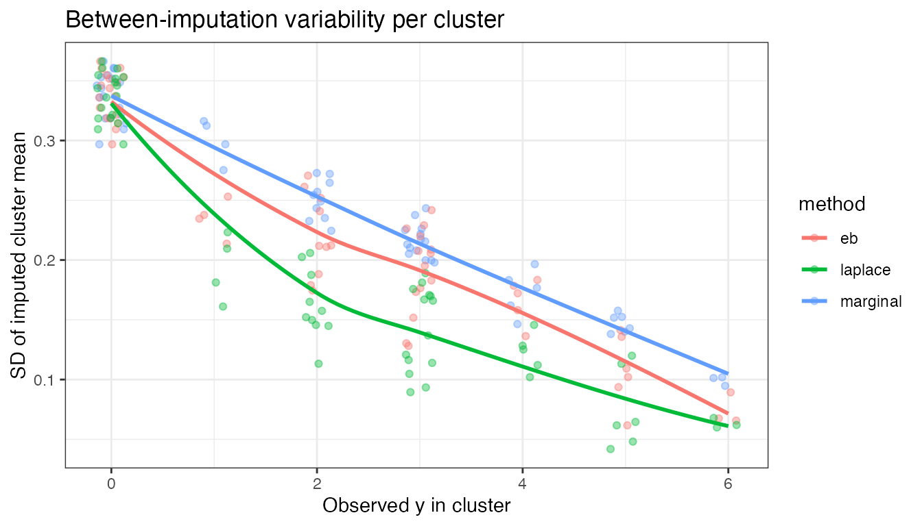

For clusters with zero observed $y$ (systematic, $n_\text{obs} = 0$), all three methods draw from the marginal prior and are identical. As $n_\text{obs}$ increases:

• "marginal" stays high — it ignores the observed data within the cluster and always draws from the prior.
• "eb" drops — it centres on the BLUP, but uses the full prior width, so variability stays moderate.
• "laplace" drops fastest — it uses both the BLUP and the tighter posterior variance, giving the most precise draws for well-observed clusters.

Cluster-level bias

true_cluster_p <- tapply(plogis(logit), cluster, mean)

get_bias <- function(imp, label) {
  mean_imp <- rowMeans(sapply(seq_len(imp$m), function(i) {
    tapply(complete(imp, i)$y_miss, complete(imp, i)$cluster, mean)
  }))
  data.frame(
    method   = label,
    true_p   = true_cluster_p,
    imp_mean = mean_imp,
    n_obs    = as.numeric(n_obs_per_cluster)
  )
}

bias <- rbind(
  get_bias(imp_marginal, "marginal"),
  get_bias(imp_eb,       "eb"),
  get_bias(imp_laplace,  "laplace")
)

ggplot(bias, aes(x = true_p, y = imp_mean, colour = n_obs)) +
  geom_point(alpha = 0.6) +
  geom_abline(slope = 1, intercept = 0, linetype = "dashed") +
  facet_wrap(~method) +
  scale_colour_viridis_c(name = "n obs") +
  labs(x = "True cluster probability", y = "Mean imputed cluster probability",
       title = "Imputed vs true cluster probability") +
  theme_bw()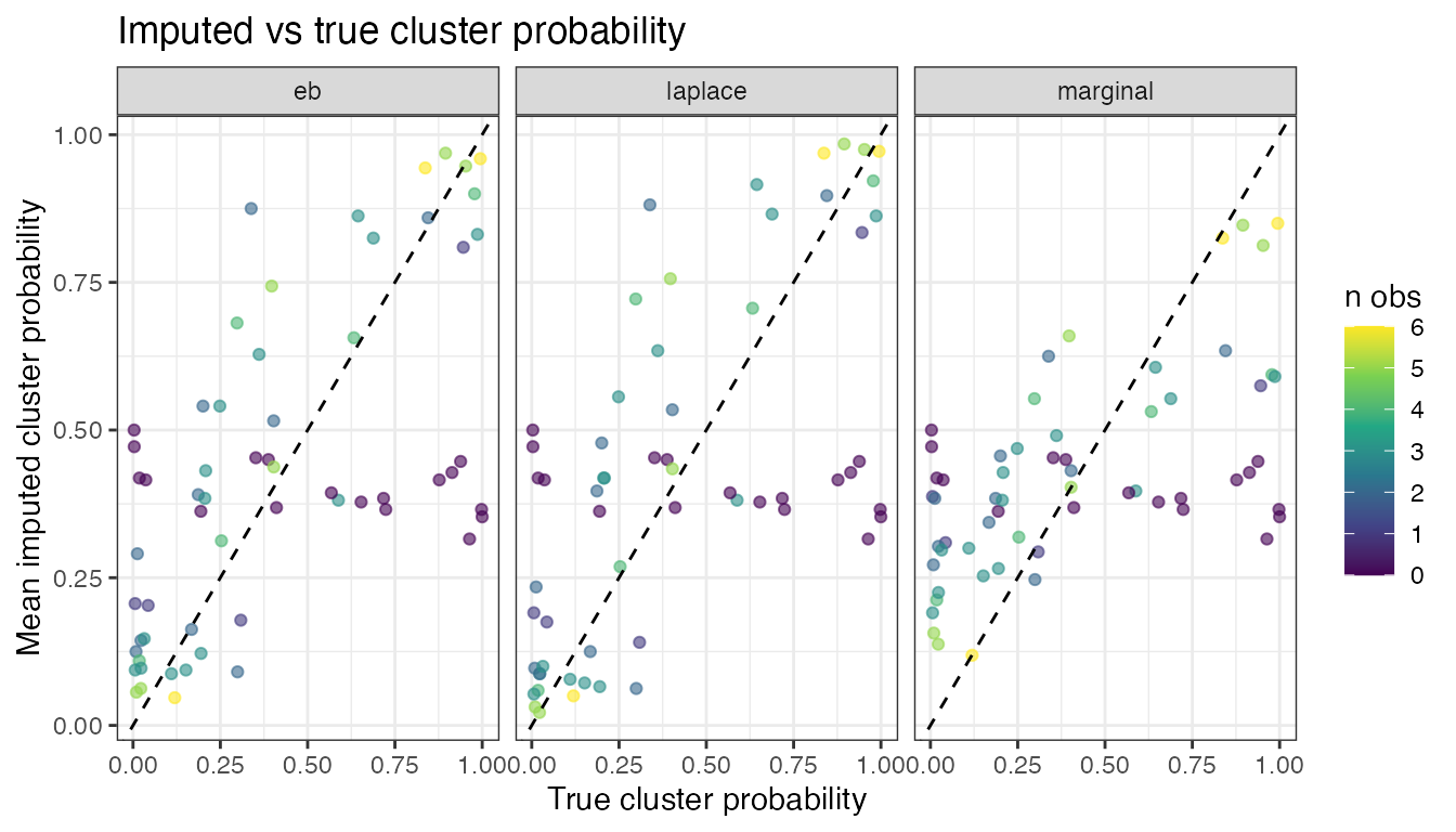

"laplace" and "eb" track the true cluster probabilities more closely than "marginal", particularly for extreme clusters (high or low true probability). "marginal" shows shrinkage toward the population mean because it ignores the cluster’s own observed data.

Recommendation

Use random.effects = "laplace" (the default) for most applications. It is the only method that correctly handles the full spectrum from sporadic to systematic missingness within a single coherent framework.

Use random.effects = "marginal" only if all missing clusters are known to be systematically missing (no observed $y$ in the cluster at all).

Use random.effects = "eb" as a fast approximation when clusters are large (many observations per cluster), so that posterior uncertainty in $\hat{b}_i$ is small relative to $\psi^*$.

References

Audigier, V., White, I. R., Jolani, S., Debray, T. P. A., Quartagno, M., Carpenter, J., van Buuren, S., & Resche-Rigon, M. (2018). Multiple imputation for multilevel data with continuous and binary variables. Statistical Science, 33(2), 160–183. https://doi.org/10.1214/18-STS646