Walking disability data

Two items YA and YB measuring walking disability in samples A, B and E.

Format

A data frame with 890 rows on the following 5 variables:

sex

Sex of respondent (factor)

age

Age of respondent

YA

Item administered in samples A and E (factor)

YB

Item administered in samples B and E (factor)

src

Source: Sample A, B or E (factor)

Details

Example dataset to demonstrate imputation of two items (YA and YB). Item YA is administered to sample A and sample E, item YB is administered to sample B and sample E, so sample E acts as a bridge study. Imputation using a bridge study is better than simple equating or than imputation under independence.

Item YA corresponds to the HAQ8 item, and item YB corresponds to the GAR9 items from Van Buuren et al (2005). Sample E (as well as sample B) is the Euridiss study (n=292), sample A is the ERGOPLUS study (n=306).

See Van Buuren (2018) section 9.4 for more details on the imputation methodology.

References

van Buuren, S., Eyres, S., Tennant, A., Hopman-Rock, M. (2005). Improving comparability of existing data by Response Conversion. Journal of Official Statistics, 21(1), 53-72.

Van Buuren, S. (2018). Flexible Imputation of Missing Data. Second Edition. Chapman & Hall/CRC. Boca Raton, FL.

Examples

md.pattern(walking)

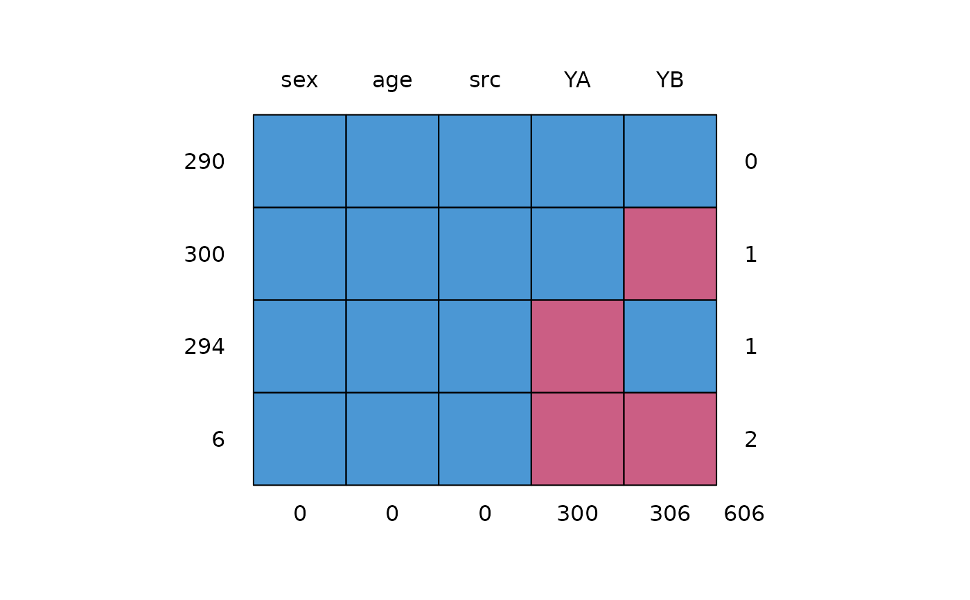#>     sex age src  YA  YB    
#> 290   1   1   1   1   1   0
#> 300   1   1   1   1   0   1
#> 294   1   1   1   0   1   1
#> 6     1   1   1   0   0   2
#>       0   0   0 300 306 606

micemill <- function(n) {
  for (i in 1:n) {
    imp <<- mice.mids(imp) # global assignment
    cors <- with(imp, cor(as.numeric(YA),
      as.numeric(YB),
      method = "kendall"
    ))
    tau <<- rbind(tau, getfit(cors, s = TRUE)) # global assignment
  }
}

plotit <- function() {
  matplot(
    x = 1:nrow(tau), y = tau,
    ylab = expression(paste("Kendall's ", tau)),
    xlab = "Iteration", type = "l", lwd = 1,
    lty = 1:10, col = "black"
  )
}

tau <- NULL
imp <- mice(walking, max = 0, m = 10, seed = 92786)
pred <- imp$pred
pred[, c("src", "age", "sex")] <- 0
imp <- mice(walking, max = 0, m = 3, seed = 92786, pred = pred)
micemill(5)
#> 
#>  iter imp variable
#>   1   1  YA  YB
#>   1   2  YA  YB
#>   1   3  YA  YB
#> 
#>  iter imp variable
#>   2   1  YA  YB
#>   2   2  YA  YB
#>   2   3  YA  YB
#> 
#>  iter imp variable
#>   3   1  YA  YB
#>   3   2  YA  YB
#>   3   3  YA  YB
#> 
#>  iter imp variable
#>   4   1  YA  YB
#>   4   2  YA  YB
#>   4   3  YA  YB
#> 
#>  iter imp variable
#>   5   1  YA  YB
#>   5   2  YA  YB
#>   5   3  YA  YB
plotit()


### to get figure 9.8 van Buuren (2018) use m=10 and micemill(20)