Parallel imputation: benchmarks

Introduction

This vignette measures when running the chains in parallel pays off, and compares mice(parallel = TRUE) with sequential mice() and with the wrapper futuremice() (Volker and Vink 2022). It follows the design of Volker and Vink (2022), and adds a slow imputation method and more numbers of imputations. The vignette Parallel imputation explains how to use parallel = TRUE.

The timings were computed beforehand with the script data-raw/parallel-benchmark.R in the source of the package, and are read from a file. They depend on the machine, so treat them as an indication of the pattern, not as absolute numbers. The results below were obtained on:

Item	Value
Date	2026-11-11
CPU	Apple M4 Pro
Cores	14
R	R version 4.5.2 (2025-10-31)
mice	3.19.12
future	1.75.0

Design

The data are drawn from a multivariate normal distribution with zero means, unit variances and correlations of 0.5. Eighty percent of the cases get missing values, completely at random (MCAR), by ampute(). There are three scenarios:

Scenario	Description
small	Small: 1000 x 4, pmm
large	Large: 10000 x 8, pmm
slow	Slow method: 2000 x 8, rf

The rf method fits a random forest with the ranger package for every variable in every iteration, which makes it much slower than pmm. ranger uses two threads by default, also within a worker. All runs use maxit = 5, and every combination is repeated 3 times; the figures show the median time. We compare:

mice(): the sequential sampler, on one core.
mice(parallel = TRUE): the parallel sampler, on a multisession plan with 2, 4 or 8 workers that was started before the timing, so that the workers are reused. This is how you would use it for repeated imputations (see below for the cost of starting workers).
futuremice(): the wrapper with n.core set to 2, 4 or 8. It starts and closes its own workers in every call, so these timings include the start-up of the workers.

Starting the workers

Each worker is a separate R session. A new worker has to start R and load mice and its dependencies before it can impute. The table shows the median time of a tiny imputation on new workers (cold) and on workers that are already running (warm):

Workers	Cold (s)	Warm (s)	Start-up (s)
2	0.76	0.03	0.73
4	0.84	0.04	0.80
8	0.94	0.05	0.89

Starting the workers costs about 0.8 seconds per call on this machine. mice(parallel = TRUE, n.core = 4) pays this cost in every call, as does futuremice(). Setting up the workers once with future::plan(multisession, workers = 4) pays it only for the first call. For a single long imputation the difference does not matter, but for many short imputations, for example in a simulation study, it does.

Results

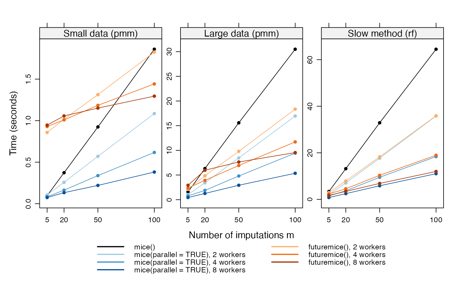
Median time (seconds) against the number of imputations m, per scenario and number of workers. Note the different vertical scales.

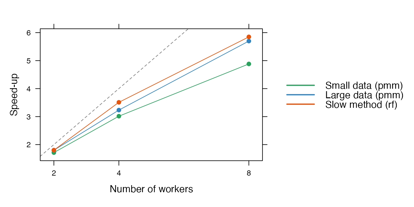
Speed-up of mice(parallel = TRUE) relative to sequential mice(), for m = 100. The dashed line is the ideal speed-up, equal to the number of workers.

When does it pay off?

Small data. For 1000 cases and 4 variables, one imputation takes a few milliseconds. Sequential mice() needs 0.10 seconds for m = 5 and 1.86 seconds for m = 100. On running workers, mice(parallel = TRUE) with 8 workers needs 0.38 seconds for m = 100. But if the workers have to be started first, the start-up cost of about 0.8 seconds is larger than the whole sequential run for small m. For small data, parallel imputation only helps with many imputations, on workers that are already running.
Large data. For 10000 cases and 8 variables, mice() takes 1.6 seconds for m = 5 and 30.5 seconds for m = 100. With 8 workers, this becomes 0.44 and 5.4 seconds, a speed-up of 5.7 for m = 100. Including the start-up of new workers, parallel imputation pays off from m = 20 on; for m = 5 the gain is small.
Slow method. With rf, mice() takes 64.5 seconds for m = 100, and mice(parallel = TRUE) with 8 workers 11.0 seconds, a speed-up of 5.8. The slower the imputation, the smaller the share of the fixed costs, and the closer the speed-up gets to the number of workers.
Number of workers. The speed-up grows with the number of workers, but less than proportionally (second figure). With m chains, at most m workers can be busy, and with m = 5 and 8 workers, three workers are idle. Each worker also has to receive the data and return its chains.

The time per chain is the same for all values of m, so a parallel run takes roughly the time of m / workers sequential chains, plus a fixed overhead. A rule of thumb: if one sequential run takes less than a few seconds, the parallel run saves little; if it takes minutes, the parallel run is close to workers times faster.

Comparison with `futuremice()`

futuremice() splits the m imputations into one block per worker, and runs a complete mice() call for each block, including its own set-up and starting imputations. The blocks are then combined with ibind(). mice(parallel = TRUE) sets up the imputation model and the starting imputations once, and only runs the chains on the workers.

For m = 100 with 8 workers, futuremice() took 9.5 seconds for the large data and 12.0 seconds for the slow method, against 5.4 and 11.0 seconds for mice(parallel = TRUE). About 0.8 seconds of the difference is the start-up of the workers, which futuremice() pays in every call. The remainder is probably due to the repeated set-up per block and the combining of the blocks. For small data, the start-up cost dominates: futuremice() is only faster than sequential mice() for m = 100 (1.30 against 1.86 seconds with 8 workers).

Moving from `futuremice()` to `mice(parallel = TRUE)`

Most arguments of futuremice() have a direct counterpart, or are no longer needed:

`futuremice()`	`mice(parallel = TRUE)`
`n.core = 4`	`n.core = 4`, or set up the workers once with `future::plan(multisession, workers = 4)`
`parallelseed = 123`	`seed = 123`
`seed` (gives identical imputations on all cores)	not needed
`use.logical = FALSE`	`future::plan(multisession, workers = parallelly::availableCores(logical = FALSE))`
`future.plan = "multicore"`	`future::plan(multicore)` before the call
`packages = "miceadds"`	not needed: methods from packages are loaded on the workers, if installed
`globals = "mice.impute.mymethod"`	not needed: user-written methods, their helper functions and objects used in `post` are sent along
`...`	`...`

The results differ in a few other ways:

Reproducibility. futuremice() gives reproducible results for a given parallelseed and n.core. mice(parallel = TRUE) gives the same imputations for a given seed, whatever the number of workers.
Plan. futuremice() sets the plan to sequential when it returns, also if you had set up workers yourself. mice(parallel = TRUE) leaves a plan set by the user untouched.
Logged events. ibind() keeps the loggedEvents of the first block only, so futuremice() drops the events logged by the other workers. mice(parallel = TRUE) collects the events of all chains.
Continuing. An object from mice(parallel = TRUE) can be continued with mice.mids(), in parallel, with the same result as a single run.
Starting imputations. futuremice() draws the starting imputations separately for each block; mice(parallel = TRUE) draws them once, as mice() does.

Reproducing the benchmark

To rerun the benchmark on your own machine, install the version of mice to test (the workers load the installed version), and run from the root of the source package:

source("data-raw/parallel-benchmark.R")

This takes about half an hour on a laptop, and writes vignettes/parallel-benchmark.rds.

References

Volker, Thom Benjamin, and Gerko Vink. 2022. futuremice: The Future Starts Today. https://www.gerkovink.com/miceVignettes/futuremice/Vignette_futuremice.html.

2026-11-11