Imputation by predictive mean matching

Usage

mice.impute.pmm(
  y,
  ry,
  x,
  wy = NULL,
  donors = 5L,
  matchtype = 1L,
  exclude = NULL,
  quantify = TRUE,
  trim = 1L,
  ridge = 1e-05,
  use.matcher = FALSE,
  ...
)

Arguments

y: Vector to be imputed
ry: Logical vector of length length(y) indicating the the subset y[ry] of elements in y to which the imputation model is fitted. The ry generally distinguishes the observed (TRUE) and missing values (FALSE) in y.
x: Numeric design matrix with length(y) rows with predictors for y. Matrix x may have no missing values.
wy: Logical vector of length length(y). A TRUE value indicates locations in y for which imputations are created.
donors: The size of the donor pool among which a draw is made. The default is donors = 5L. Setting donors = 1L always selects the closest match, but is not recommended. Values between 3L and 10L provide the best results in most cases (Morris et al, 2015).
matchtype: Type of matching distance. The default choice (matchtype = 1L) calculates the distance between the predicted value of yobs and the drawn values of ymis (called type-1 matching). Other choices are matchtype = 0L (distance between predicted values) and matchtype = 2L (distance between drawn values).
exclude: Dependent values to exclude from the imputation model and the collection of donor values
quantify: Logical. If TRUE, factor levels are replaced by the first canonical variate before fitting the imputation model. If false, the procedure reverts to the old behaviour and takes the integer codes (which may lack a sensible interpretation). Relevant only of y is a factor.
trim: Scalar integer. Minimum number of observations required in a category in order to be considered as a potential donor value. Relevant only of y is a factor.
ridge: The ridge penalty used in .norm.draw() to prevent problems with multicollinearity. The default is ridge = 1e-05, which means that 0.01 percent of the diagonal is added to the cross-product. Larger ridges may result in more biased estimates. For highly noisy data (e.g. many junk variables), set ridge = 1e-06 or even lower to reduce bias. For highly collinear data, set ridge = 1e-04 or higher.
use.matcher: Logical. Set use.matcher = TRUE to specify the C function matcher(), the now deprecated matching function that was default in versions 2.22 (June 2014) to 3.11.7 (Oct 2020). Since version 3.12.0 mice() uses the much faster matchindex C function. Use the deprecated matcher function only for exact reproduction.
...: Other named arguments.

Value

Vector with imputed data, same type as y, and of length sum(wy)

Details

Imputation of y by predictive mean matching, based on van Buuren (2012, p. 73). The procedure is as follows:

Calculate the cross-product matrix \(S=X_{obs}'X_{obs}\).
Calculate \(V = (S+{diag}(S)\kappa)^{-1}\), with some small ridge parameter \(\kappa\).
Calculate regression weights \(\hat\beta = VX_{obs}'y_{obs}.\)
Draw \(q\) independent \(N(0,1)\) variates in vector \(\dot z_1\).
Calculate \(V^{1/2}\) by Cholesky decomposition.
Calculate \(\dot\beta = \hat\beta + \dot\sigma\dot z_1 V^{1/2}\).
Calculate \(\dot\eta(i,j)=|X_{{obs},[i]|}\hat\beta-X_{{mis},[j]}\dot\beta\) with \(i=1,\dots,n_1\) and \(j=1,\dots,n_0\).
Construct \(n_0\) sets \(Z_j\), each containing \(d\) candidate donors, from Y_obs such that \(\sum_d\dot\eta(i,j)\) is minimum for all \(j=1,\dots,n_0\). Break ties randomly.
Draw one donor \(i_j\) from \(Z_j\) randomly for \(j=1,\dots,n_0\).
Calculate imputations \(\dot y_j = y_{i_j}\) for \(j=1,\dots,n_0\).

The name predictive mean matching was proposed by Little (1988).

References

Little, R.J.A. (1988), Missing data adjustments in large surveys (with discussion), Journal of Business Economics and Statistics, 6, 287--301.

Morris TP, White IR, Royston P (2015). Tuning multiple imputation by predictive mean matching and local residual draws. BMC Med Res Methodol. ;14:75.

Van Buuren, S. (2018). Flexible Imputation of Missing Data. Second Edition. Chapman & Hall/CRC. Boca Raton, FL.

Van Buuren, S., Groothuis-Oudshoorn, K. (2011). mice: Multivariate Imputation by Chained Equations in R. Journal of Statistical Software, 45(3), 1-67. doi:10.18637/jss.v045.i03

Author

Gerko Vink, Stef van Buuren, Karin Groothuis-Oudshoorn

Examples

# We normally call mice.impute.pmm() from within mice()
# But we may call it directly as follows (not recommended)

set.seed(53177)
xname <- c("age", "hgt", "wgt")
r <- stats::complete.cases(boys[, xname])
x <- boys[r, xname]
y <- boys[r, "tv"]
ry <- !is.na(y)
table(ry)
#> ry
#> FALSE  TRUE 
#>   503   224 

# percentage of missing data in tv
sum(!ry) / length(ry)
#> [1] 0.6918845

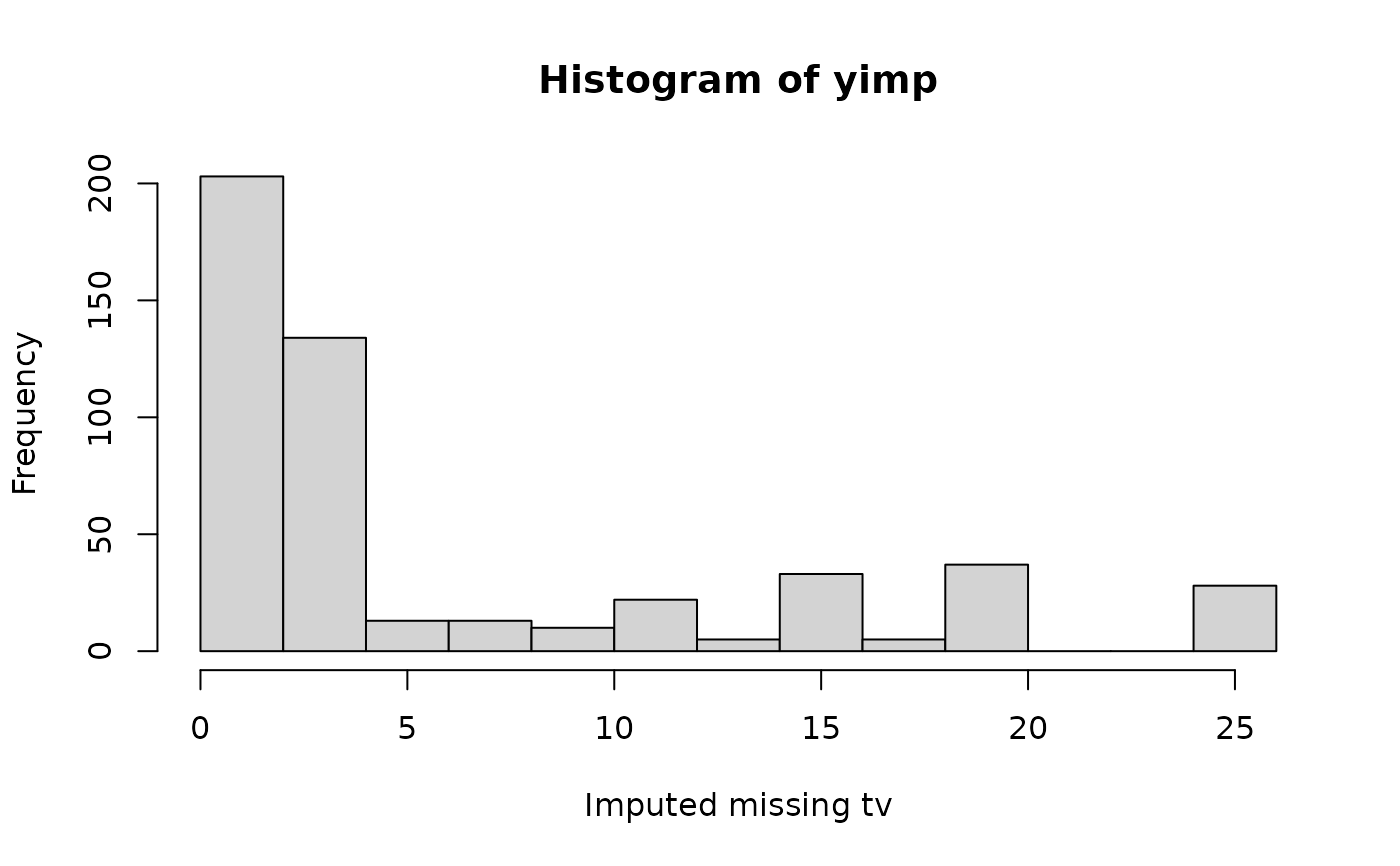
# Impute missing tv data
yimp <- mice.impute.pmm(y, ry, x)
length(yimp)
#> [1] 503
hist(yimp, xlab = "Imputed missing tv")


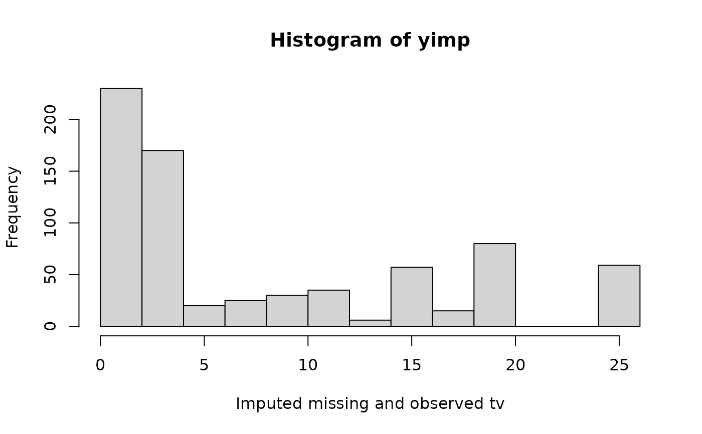
# Impute all tv data
yimp <- mice.impute.pmm(y, ry, x, wy = rep(TRUE, length(y)))
length(yimp)
#> [1] 727
hist(yimp, xlab = "Imputed missing and observed tv")

plot(jitter(y), jitter(yimp),
  main = "Predictive mean matching on age, height and weight",
  xlab = "Observed tv (n = 224)",
  ylab = "Imputed tv (n = 224)"
)
abline(0, 1)

cor(y, yimp, use = "pair")
#> [1] 0.7415001

# Use blots to exclude different values per column
# Create blots object
blots <- make.blots(boys)
# Exclude ml 1 through 5 from tv donor pool
blots$tv$exclude <- c(1:5)
# Exclude 100 random observed heights from tv donor pool
blots$hgt$exclude <- sample(unique(boys$hgt), 100)
imp <- mice(boys, method = "pmm", print = FALSE, blots = blots, seed=123)
blots$hgt$exclude %in% unlist(c(imp$imp$hgt)) # MUST be all FALSE
#>   [1] FALSE FALSE FALSE FALSE FALSE FALSE FALSE FALSE FALSE FALSE FALSE FALSE
#>  [13] FALSE FALSE FALSE FALSE FALSE FALSE FALSE FALSE FALSE FALSE FALSE FALSE
#>  [25] FALSE FALSE FALSE FALSE FALSE FALSE FALSE FALSE FALSE FALSE FALSE FALSE
#>  [37] FALSE FALSE FALSE FALSE FALSE FALSE FALSE FALSE FALSE FALSE FALSE FALSE
#>  [49] FALSE FALSE FALSE FALSE FALSE FALSE FALSE FALSE FALSE FALSE FALSE FALSE
#>  [61] FALSE FALSE FALSE FALSE FALSE FALSE FALSE FALSE FALSE FALSE FALSE FALSE
#>  [73] FALSE FALSE FALSE FALSE FALSE FALSE FALSE FALSE FALSE FALSE FALSE FALSE
#>  [85] FALSE FALSE FALSE FALSE FALSE FALSE FALSE FALSE FALSE FALSE FALSE FALSE
#>  [97] FALSE FALSE FALSE FALSE
blots$tv$exclude %in% unlist(c(imp$imp$tv)) # MUST be all FALSE
#> [1] FALSE FALSE FALSE FALSE FALSE

# Factor quantification
xname <- c("age", "hgt", "wgt")
br <- boys[c(1:10, 101:110, 501:510, 601:620, 701:710), ]
r <- stats::complete.cases(br[, xname])
x <- br[r, xname]
y <- factor(br[r, "tv"])
ry <- !is.na(y)
table(y)
#> y
#>  6  8 10 12 13 15 16 20 25 
#>  1  2  1  1  1  4  1  4  7 

# impute factor by optimizing canonical correlation y, x
mice.impute.pmm(y, ry, x)
#>  [1] 25 25 25 20 25 25 20 25 25 25 15 25 25 25 25 25 15 15 25 15 20 15 8  25 8 
#> [26] 25 20 20 15 25 25 15 15 25 25 15 20 8 
#> Levels: 6 8 10 12 13 15 16 20 25

# only categories with at least 2 cases can be donor
mice.impute.pmm(y, ry, x, trim = 2L)
#>  [1] 8  25 25 8  8  20 15 20 20 8  8  8  15 8  20 20 15 8  20 25 20 25 20 15 20
#> [26] 20 20 20 15 20 15 25 20 25 25 20 20 20
#> Levels: 6 8 10 12 13 15 16 20 25

# in addition, eliminate category 20
mice.impute.pmm(y, ry, x, trim = 2L, exclude = 20)
#>  [1] 8  25 15 25 15 8  8  25 25 25 8  15 15 8  8  8  25 25 25 25 15 8  8  15 15
#> [26] 25 15 8  15 15 25 25 15 25 25 15 25 25
#> Levels: 6 8 10 12 13 15 16 20 25

# to get old behavior: as.integer(y))
mice.impute.pmm(y, ry, x, quantify = FALSE)
#>  [1] 8  6  10 15 12 8  6  15 15 10 10 6  8  10 8  15 8  15 8  15 15 12 15 8  20
#> [26] 25 12 25 15 25 25 13 8  20 16 20 20 20
#> Levels: 6 8 10 12 13 15 16 20 25