Create the ggmice equivalent of mice
plots
How to re-create the output of the plotting functions from
mice with ggmice. In alphabetical order of the
mice functions.
First load the ggmice, mice, and
ggplot2 packages, some incomplete data and a
mids object into your workspace.
bwplot
Box-and-whisker plot of observed and imputed data.
# original plot
mice::bwplot(imp, hgt ~ .imp)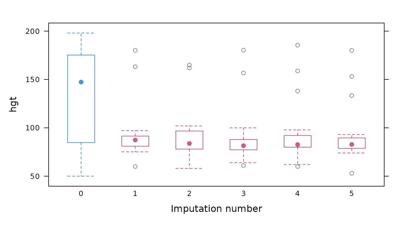
# ggmice equivalent
ggmice(imp, aes(x = .imp, y = hgt)) +
  geom_boxplot() +
  labs(x = "Imputation number")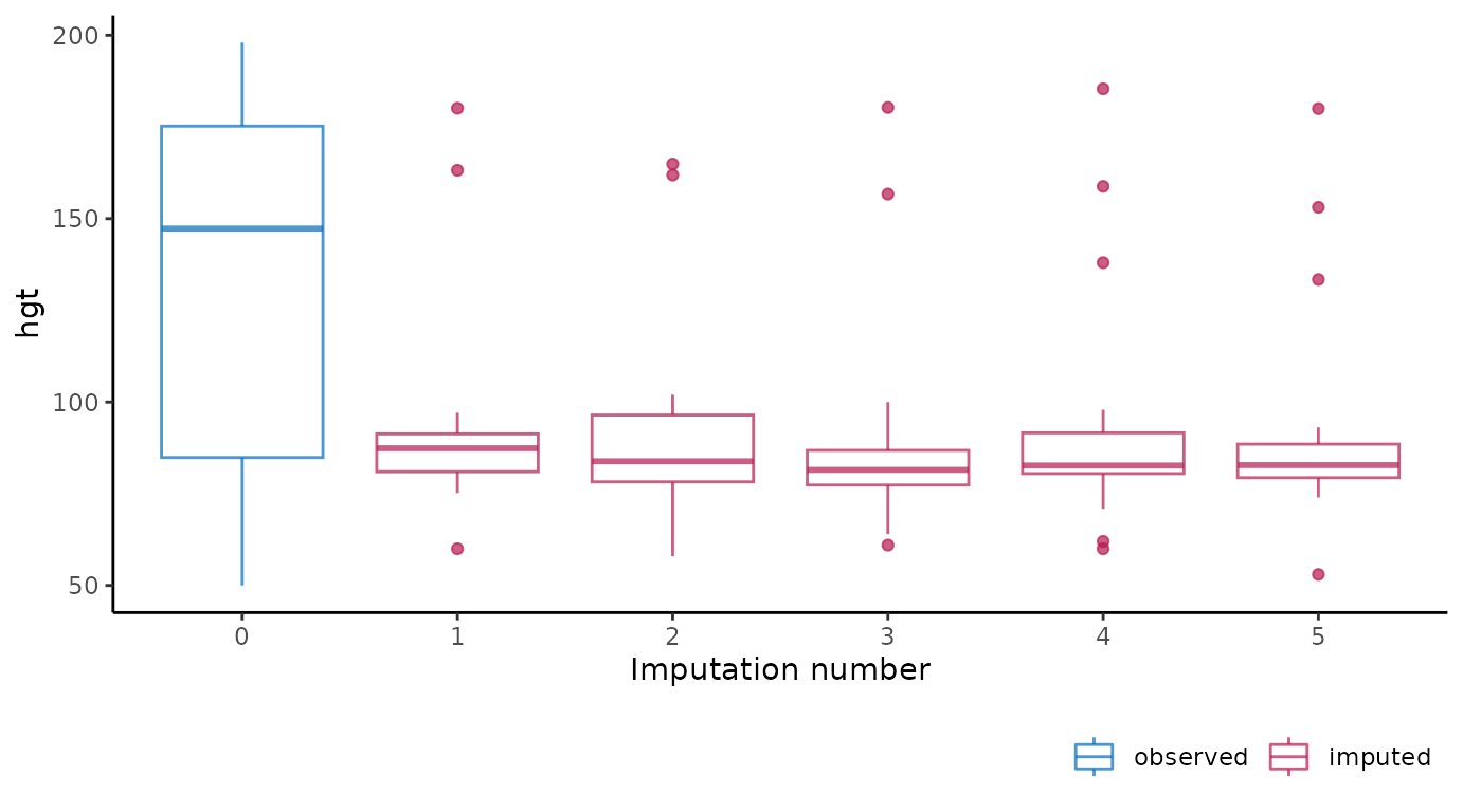
# extended reproduction with ggmice
ggmice(imp, aes(x = .imp, y = hgt)) +
  stat_boxplot(geom = "errorbar", linetype = "dashed") +
  geom_boxplot(outlier.colour = "grey", outlier.shape = 1) +
  labs(x = "Imputation number") +
  theme(legend.position = "none")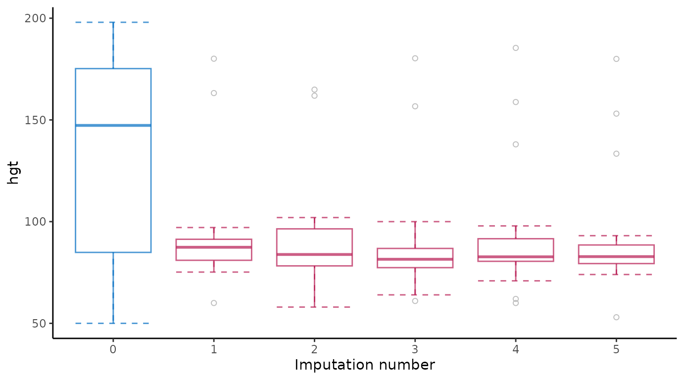
densityplot
Density plot of observed and imputed data.
# original plot
mice::densityplot(imp, ~hgt)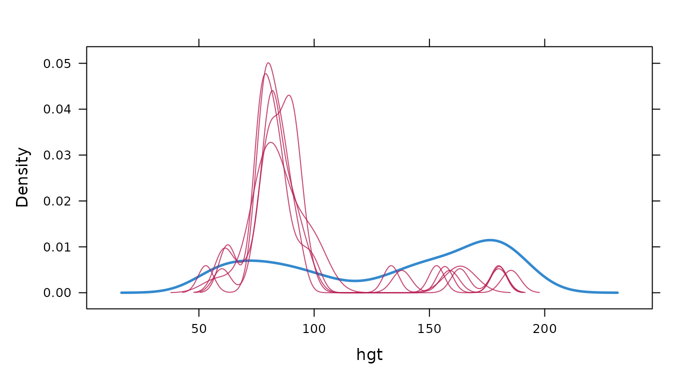
# ggmice equivalent
ggmice(imp, aes(x = hgt, group = .imp)) +
  geom_density()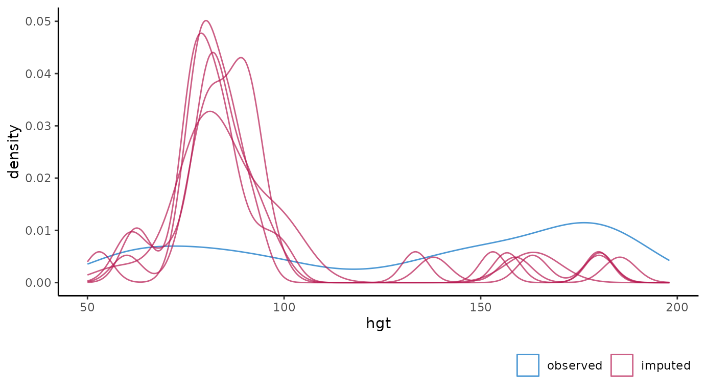
# extended reproduction with ggmice
ggmice(imp, aes(x = hgt, group = .imp, linewidth = .where)) +
  geom_density() +
  scale_linewidth_manual(
    values = c("observed" = 1, "imputed" = 0.5),
    guide = "none"
  ) +
  theme(legend.position = "none")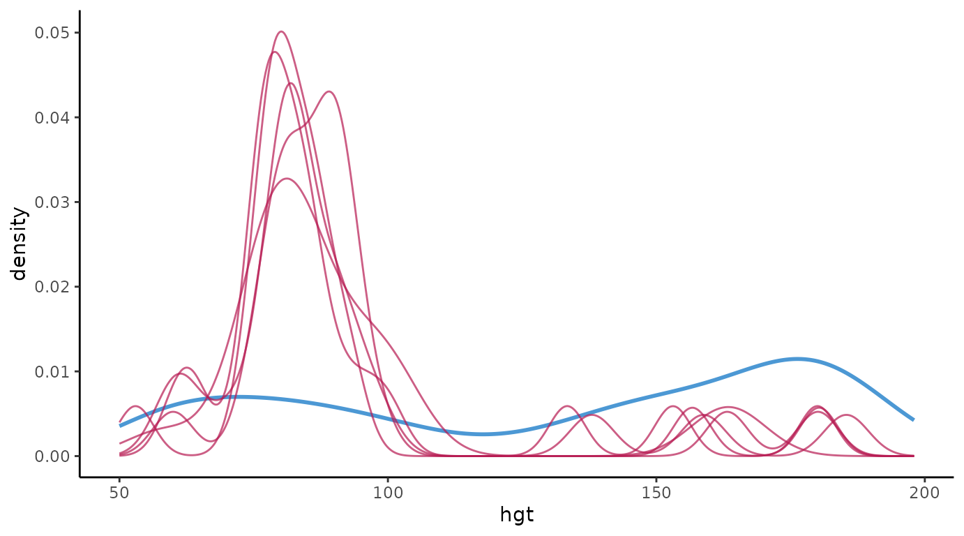
fluxplot
Influx and outflux plot of multivariate missing data patterns.
# original plot
fluxplot(dat)
# ggmice equivalent
plot_flux(dat)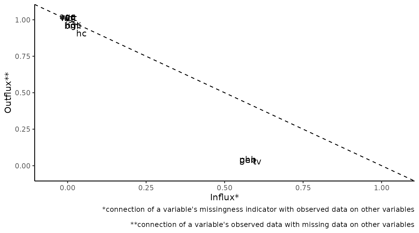
md.pattern
Missing data pattern plot.
# original plot
md <- md.pattern(dat)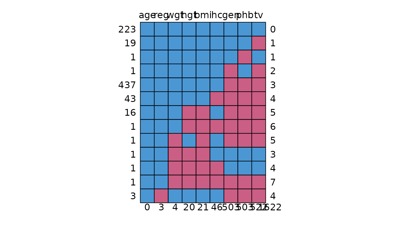
# ggmice equivalent
plot_pattern(dat)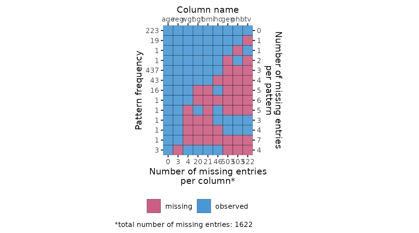
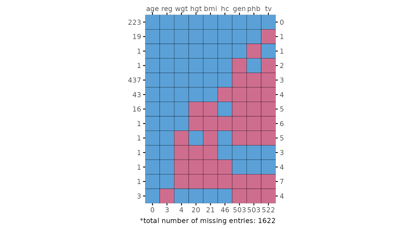
# extended reproduction with ggmice
plot_pattern(dat, square = TRUE) +
  theme(
    legend.position = "none",
    axis.title = element_blank(),
    axis.title.x.top = element_blank(),
    axis.title.y.right = element_blank()
  )
plot.mids
Plot the trace lines of the MICE algorithm.
# original plot
plot(imp, hgt ~ .it | .ms)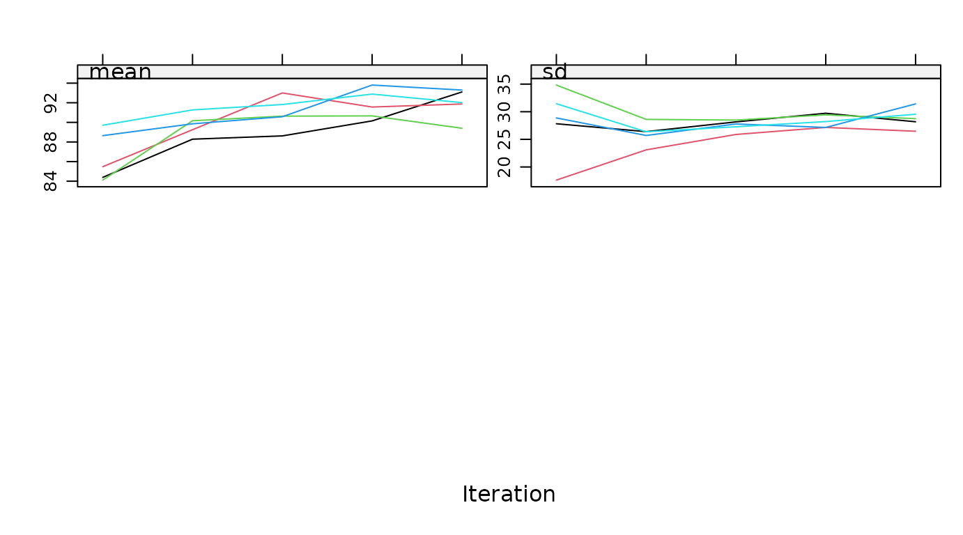
# ggmice equivalent
plot_trace(imp, "hgt")
stripplot
Stripplot of observed and imputed data.
# original plot
mice::stripplot(imp, hgt ~ .imp)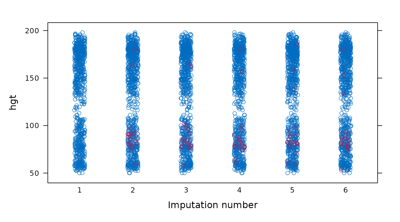
# ggmice equivalent
ggmice(imp, aes(x = .imp, y = hgt)) +
  geom_jitter(width = 0.25) +
  labs(x = "Imputation number")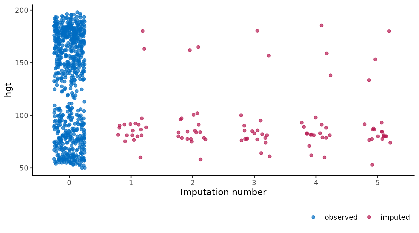
# extended reproduction with ggmice (not recommended)
ggmice(imp, aes(x = .imp, y = hgt)) +
  geom_jitter(
    shape = 1,
    width = 0.1,
    na.rm = TRUE,
    data = data.frame(
      hgt = dat$hgt,
      .imp = factor(rep(1:imp$m, each = nrow(dat))),
      .where = "observed"
    )
  ) +
  geom_jitter(shape = 1, width = 0.1) +
  labs(x = "Imputation number") +
  theme(legend.position = "none")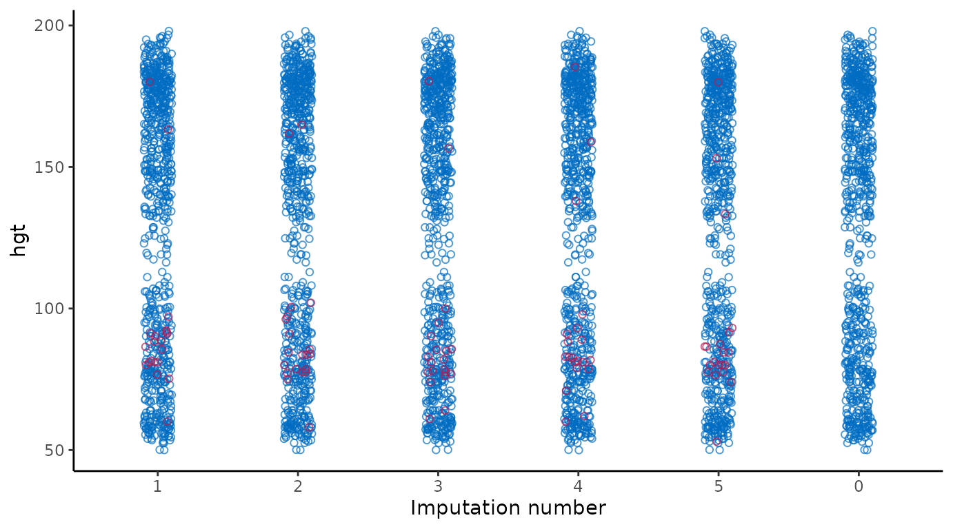
xyplot
Scatterplot of observed and imputed data.
# original plot
mice::xyplot(imp, hgt ~ age)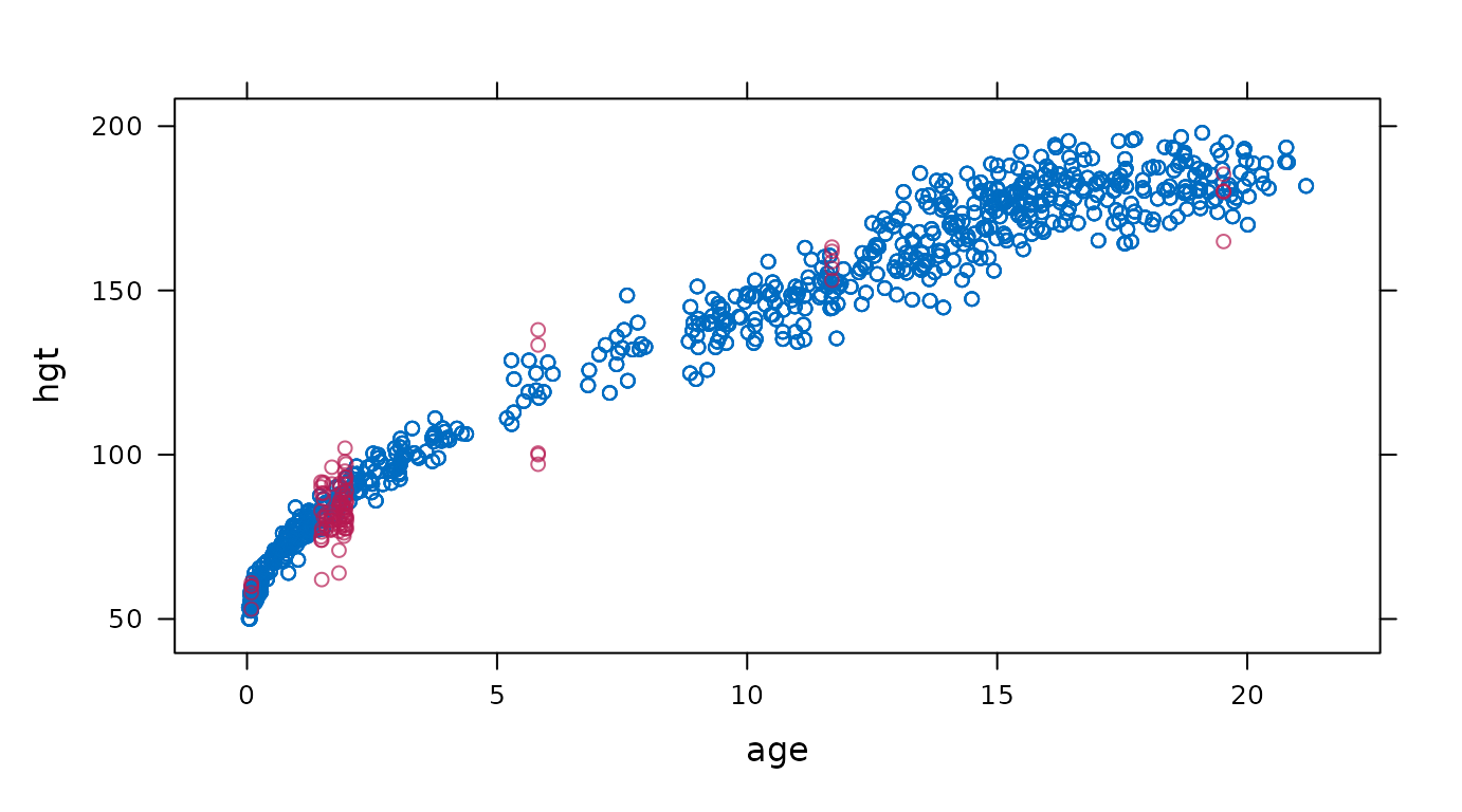
# ggmice equivalent
ggmice(imp, aes(age, hgt)) +
  geom_point()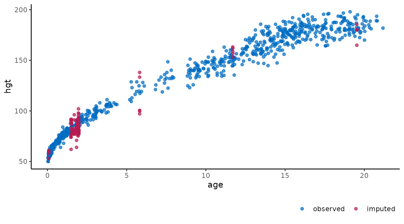
# extended reproduction with ggmice
ggmice(imp, aes(age, hgt)) +
  geom_point(size = 2, shape = 1) +
  theme(legend.position = "none")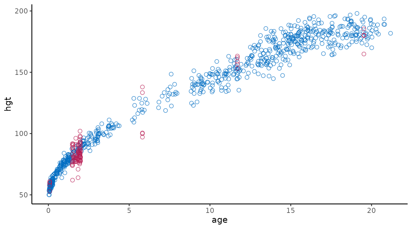
Extensions
Interactive plots
To make ggmice visualizations interactive, the
plotly package can be used. For example, an interactive
influx and outflux plot may be more legible than a static one.
Plot multiple variables
You may want to create a plot visualizing the imputations of multiple
variables as one object. To visualize multiple variables at once, the
variable names are saved in a vector. This vector is used together with
the functional programming package purrr and visualization
package patchwork to map() over the variables
and subsequently wrap_plots to create a single figure.
# load packages
library(purrr)
library(patchwork)
# create vector with variable names
vrb <- names(dat)
Display box-and-whisker plots for all variables.
# original plot
mice::bwplot(imp)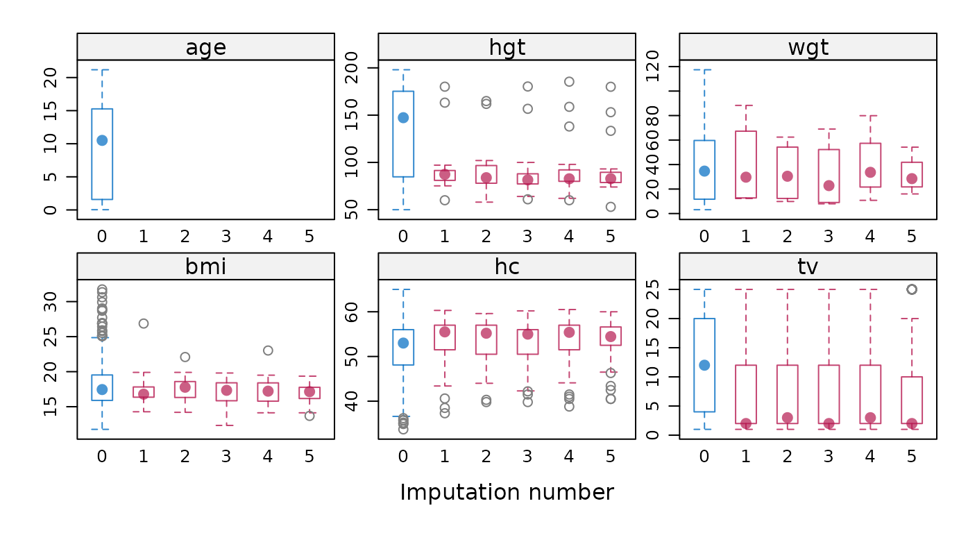
# ggmice equivalent
p <- map(vrb, ~ {
  ggmice(imp, aes(x = .imp, y = .data[[.x]])) +
    geom_boxplot() +
    scale_x_discrete(drop = FALSE) +
    labs(x = "Imputation number")
})
wrap_plots(p, guides = "collect") &
  theme(legend.position = "bottom")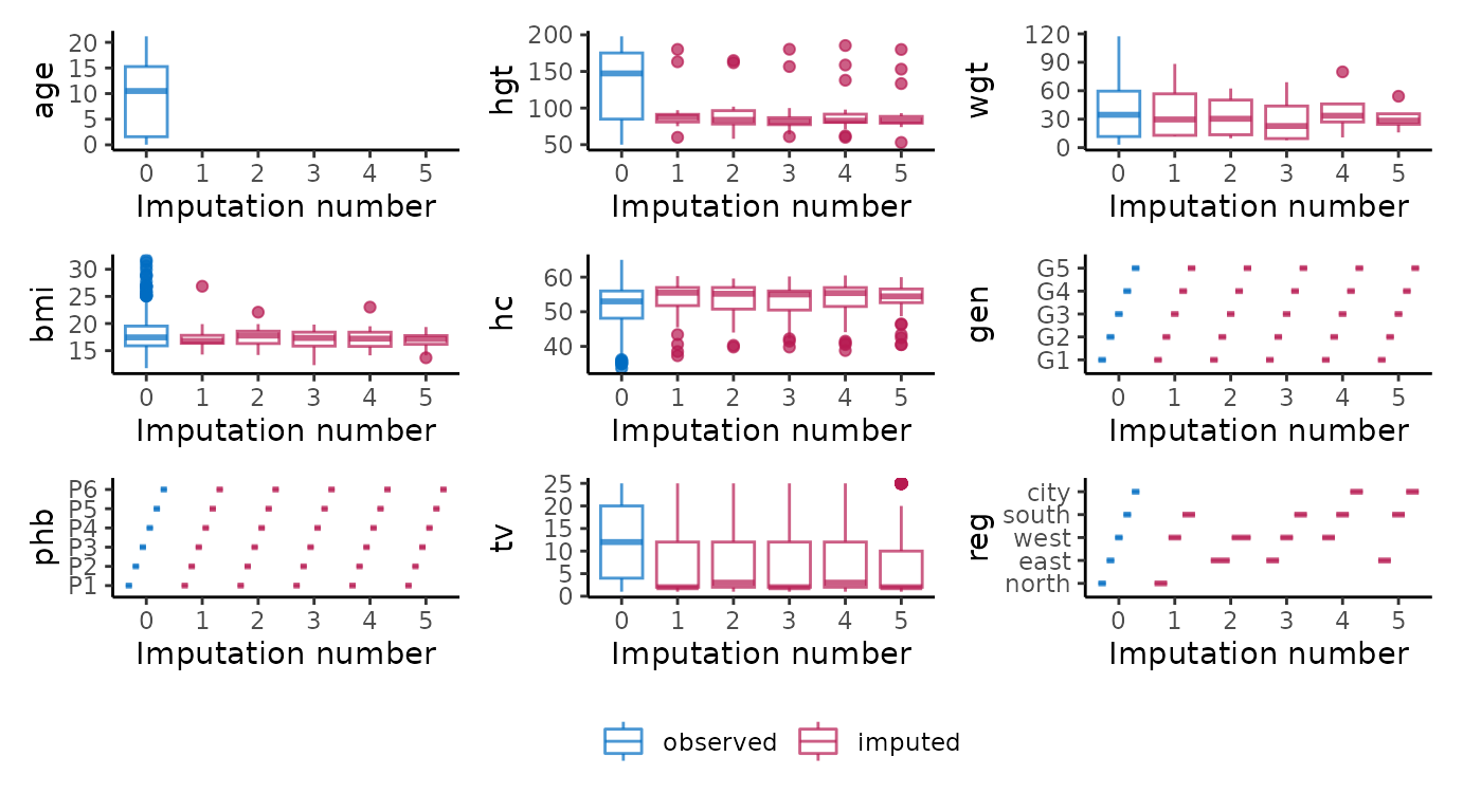
Display density plots for all variables.
# original plot
mice::densityplot(imp)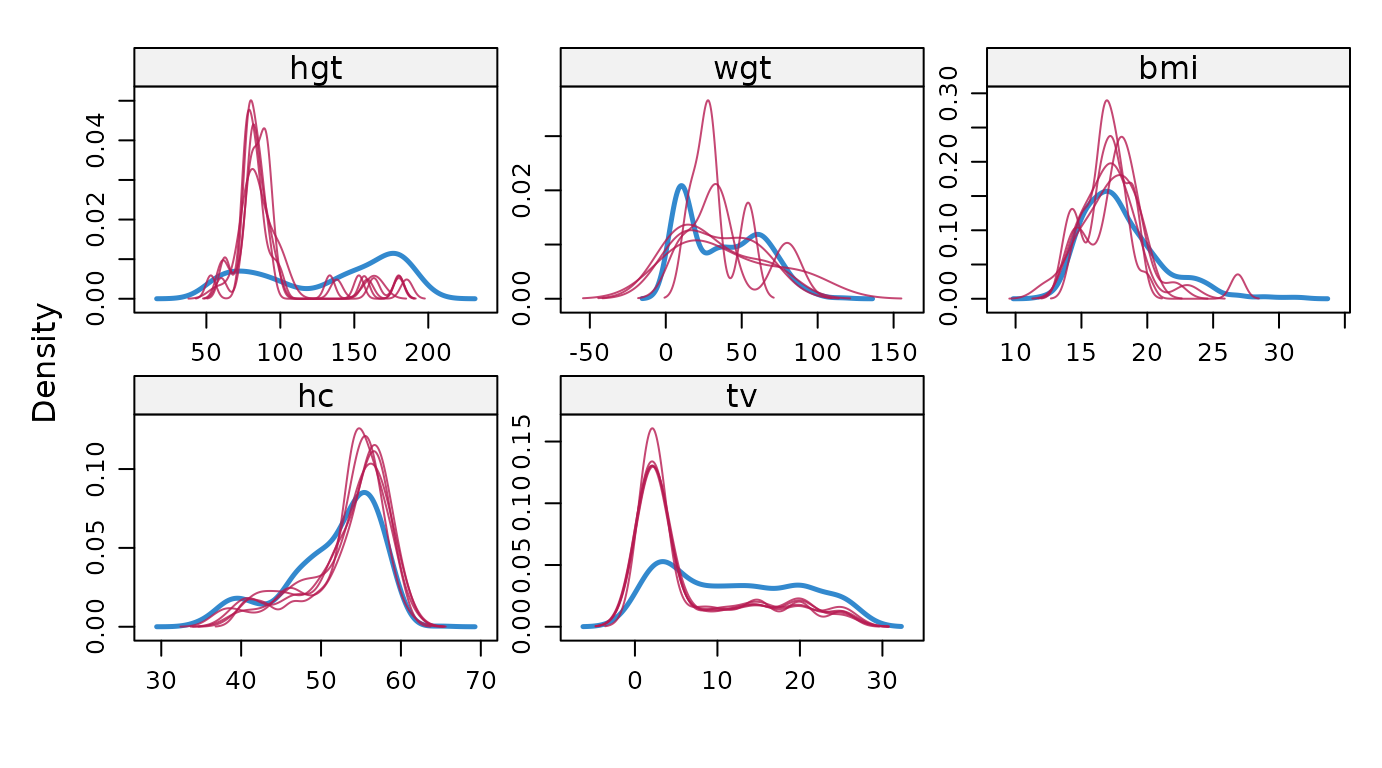
# ggmice equivalent
p <- map(vrb, ~ {
  ggmice(imp, aes(x = .data[[.x]], group = .imp)) +
    geom_density()
})
wrap_plots(p, guides = "collect") &
  theme(legend.position = "bottom")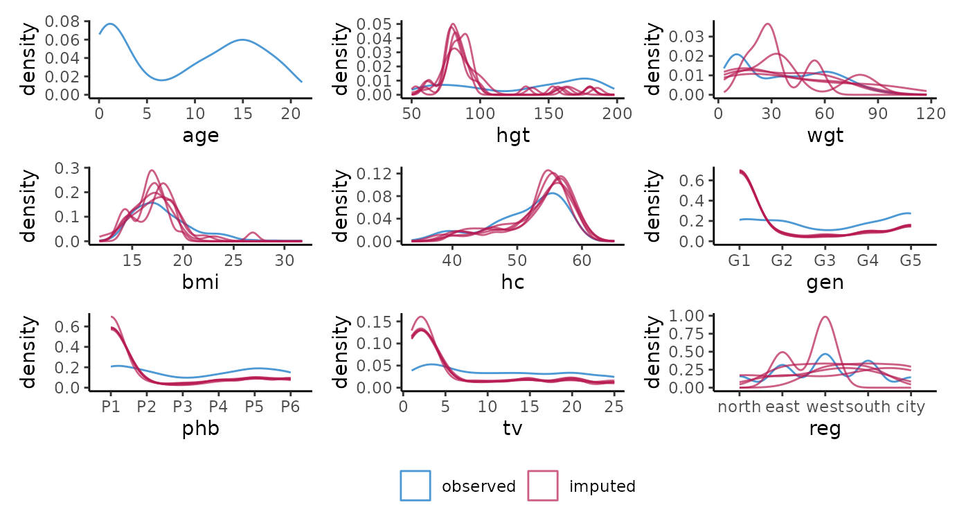
Display strip plots for all variables.
# original plot
mice::stripplot(imp)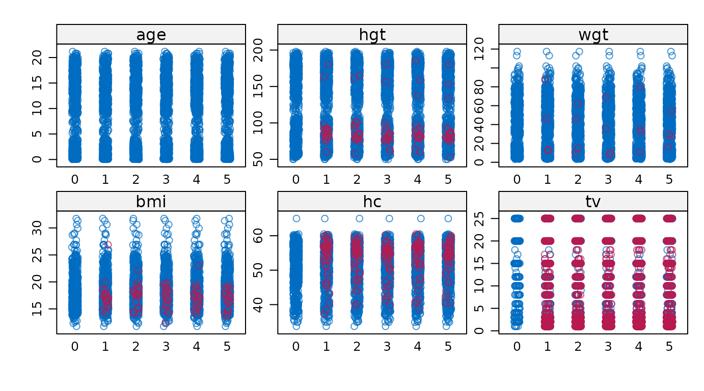
# ggmice equivalent
p <- map(vrb, ~ {
  ggmice(imp, aes(x = .imp, y = .data[[.x]])) +
    geom_jitter() +
    labs(x = "Imputation number")
})
wrap_plots(p, guides = "collect") &
  theme(legend.position = "bottom")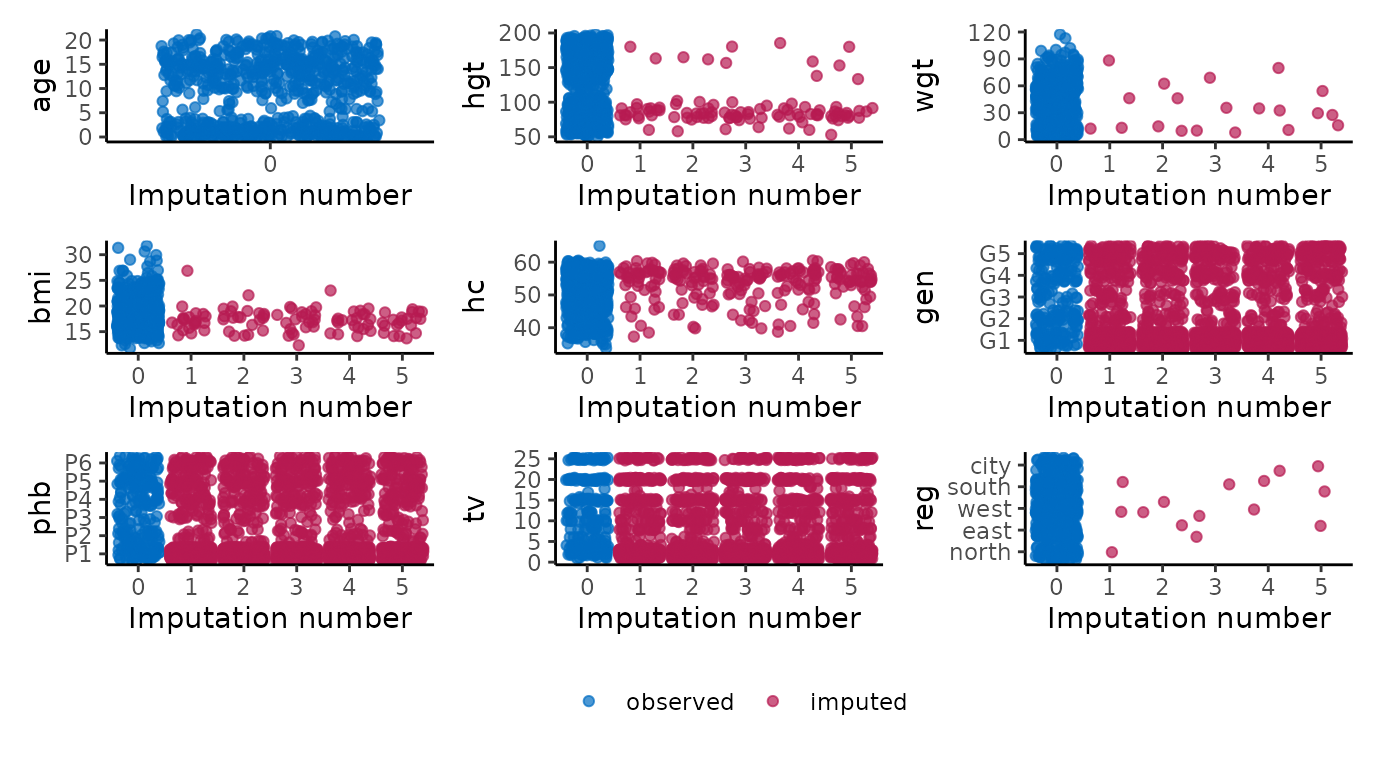
This is the end of the vignette. This document was generated using:
sessionInfo()
#> R version 4.5.3 (2026-03-11)
#> Platform: x86_64-pc-linux-gnu
#> Running under: Ubuntu 24.04.4 LTS
#>
#> Matrix products: default
#> BLAS:   /usr/lib/x86_64-linux-gnu/openblas-pthread/libblas.so.3
#> LAPACK: /usr/lib/x86_64-linux-gnu/openblas-pthread/libopenblasp-r0.3.26.so;  LAPACK version 3.12.0
#>
#> locale:
#>  [1] LC_CTYPE=C.UTF-8       LC_NUMERIC=C           LC_TIME=C.UTF-8
#>  [4] LC_COLLATE=C.UTF-8     LC_MONETARY=C.UTF-8    LC_MESSAGES=C.UTF-8
#>  [7] LC_PAPER=C.UTF-8       LC_NAME=C              LC_ADDRESS=C
#> [10] LC_TELEPHONE=C         LC_MEASUREMENT=C.UTF-8 LC_IDENTIFICATION=C
#>
#> time zone: UTC
#> tzcode source: system (glibc)
#>
#> attached base packages:
#> [1] stats     graphics  grDevices utils     datasets  methods   base
#>
#> other attached packages:
#> [1] patchwork_1.3.2   purrr_1.2.1       plotly_4.12.0     ggplot2_4.0.2
#> [5] mice_3.19.0       ggmice_0.1.1.9000
#>
#> loaded via a namespace (and not attached):
#>  [1] gtable_0.3.6        shape_1.4.6.1       xfun_0.57
#>  [4] bslib_0.10.0        htmlwidgets_1.6.4   lattice_0.22-9
#>  [7] crosstalk_1.2.2     vctrs_0.7.2         tools_4.5.3
#> [10] Rdpack_2.6.6        generics_0.1.4      tibble_3.3.1
#> [13] pan_1.9             pkgconfig_2.0.3     jomo_2.7-6
#> [16] Matrix_1.7-4        data.table_1.18.2.1 RColorBrewer_1.1-3
#> [19] S7_0.2.1            desc_1.4.3          lifecycle_1.0.5
#> [22] compiler_4.5.3      farver_2.1.2        stringr_1.6.0
#> [25] textshaping_1.0.5   codetools_0.2-20    htmltools_0.5.9
#> [28] sass_0.4.10         lazyeval_0.2.2      yaml_2.3.12
#> [31] glmnet_4.1-10       pillar_1.11.1       pkgdown_2.2.0
#> [34] nloptr_2.2.1        jquerylib_0.1.4     tidyr_1.3.2
#> [37] MASS_7.3-65         cachem_1.1.0        reformulas_0.4.4
#> [40] iterators_1.0.14    rpart_4.1.24        boot_1.3-32
#> [43] foreach_1.5.2       mitml_0.4-5         nlme_3.1-168
#> [46] tidyselect_1.2.1    digest_0.6.39       stringi_1.8.7
#> [49] dplyr_1.2.0         labeling_0.4.3      splines_4.5.3
#> [52] fastmap_1.2.0       grid_4.5.3          cli_3.6.5
#> [55] magrittr_2.0.4      survival_3.8-6      broom_1.0.12
#> [58] withr_3.0.2         scales_1.4.0        backports_1.5.0
#> [61] httr_1.4.8          rmarkdown_2.31      otel_0.2.0
#> [64] nnet_7.3-20         lme4_2.0-1          ragg_1.5.2
#> [67] evaluate_1.0.5      knitr_1.51          rbibutils_2.4.1
#> [70] viridisLite_0.4.3   rlang_1.1.7         Rcpp_1.1.1
#> [73] glue_1.8.0          minqa_1.2.8         jsonlite_2.0.0
#> [76] R6_2.6.1            systemfonts_1.3.2   fs_2.0.1